The aim of this project is to download all the ads of houses for sale in Trieste from the Idealista website and conduct a preliminary analysis of the data. Moreover, we will create a map with the location of the houses for sale, to get an idea of the distribution of the ads and their prices in the city.
Get the Data
Code
librerie =c("jsonlite","httr", # for the API"scales","ggplot2","leaflet", # for the map"RColorBrewer", # for the map"doParallel","parallel",# "reticulate", "tidymodels","tidyverse","plotly","randomForest"# for na.roughfix)# OLD functionInstall_And_Load <-function(packages) { k <- packages[!(packages %in%installed.packages()[,"Package"])];if(length(k)) {install.packages(k, repos='https://cran.rstudio.com/');}for(package_name in packages) {library(package_name,character.only=TRUE, quietly =TRUE);}}# pak::pak(librerie)# the tidyverse functions are used instead of the others in case of same name# for two functions# conflicted::conflict_prefer_all("tidyverse")conflicted::conflict_prefer_all("dplyr")conflicted::conflict_prefer_all("ggplot2")Install_And_Load(librerie)theme_set(theme_minimal())thematic::thematic_rmd()
To access the idealista APIs we need to obtain the credentials. You can get them by registering on the idealista website.
Establish the parameters for the request link. Our goal is to obtain all ads for houses for sale in Trieste. The central point is set to the center of Trieste, with a maximum distance of 10 km. We also require a minimum size of 30 square meters for the ads Establish the parameters for the request link. Our goal is to obtain all ads for houses for sale in Trieste. The central point is set to the center of Trieste, with a maximum distance of 10 km. We also require a minimum size of 30 square meters for the ads to exclude garages.to exclude garages.
Code
#url user parameters# x = '36.71145256718129' For Malaga# y = '-4.4288958904720355'x ='45.643170'y ='13.790524'maxItems ='10000'distance ='10000'type ='homes'op ='sale'minprice ='30001'maxprice ='200000000'minsize ='30'maxsize ='10000'#url fixed parameters# site = 'https://api.idealista.com/3.5/es/search?' For Spainsite ='https://api.idealista.com/3.5/it/search?'loc ='center='# country = '&country=es'country ='&country=it'maxitems ='&maxItems=50'pages ='&numPage='dist ='&distance='property ='&propertyType='operation ='&operation='pricefrom ='&minPrice='priceto ='&maxPrice='misize ='&minSize='masize ='&maxSize='chalet ='&chalet=0'
Now, we will send the request to Idealista. We have a monthly limit of 100(pagina = 100) for requests and one for second (Sys.sleep(1)). Each request is different only by the result page’s index.
Once the data are downloaded and extracted from JSON, we’ll get the lists that have to extract and put in a dataset. The problem araises becuase inside the lists are present other lists nested and not for each ad but only for someone. So that we create an empty matrix with the unique items number for ads as columns and the number of rows equal to the number of ads.
Code
pagina =100for(z in1:pagina){print(z)# prepara l'url url <-paste0(site, loc, x, ',', y, country, maxitems, pages, z, dist, distance, property, type, operation, op, pricefrom, minprice, priceto, maxprice, misize, minsize, masize, maxsize)# invia la richiesta a idealista res <- httr::POST(url, httr::add_headers("Authorization"= token))# estrai il contenuto dal JSON cont_raw <- httr::content(res) # stop the cycle if there are no more resultsif(length(cont_raw[[1]]) ==0) break# NUOVO: Prendo i nomi delle colonne da tutte le liste e li uniscomap(1:length(cont_raw[[1]]),function(x) {# the if is necessary because the list can be empty in the last pageif(length(cont_raw[[1]][[x]]) ==0) return(NULL)return(names(cont_raw[[1]][[x]])) } ) |>unlist() |>unique() -> colNames# Creo una matrice vuota dove imagazzinare i valori m =matrix(NA, nrow =length(cont_raw[[1]]), ncol =length(colNames))colnames(m) = colNamesfor(r in1:length(cont_raw[[1]])) {for(c in1:length(cont_raw[[1]][[r]])) {# nel caso l'elemento della lista sia una sotto lista o df vado a # spacchettarlo aggiungendo colonneif(length(cont_raw[[1]][[r]][[c]])>1) {# non si può fare in un unico casofor(i in1:length(cont_raw[[1]][[r]][[c]])) {# se la colonna della sottolista non è già stata aggiunta lo faccioif(is.null(names(cont_raw[[1]][[r]][[c]]))) { cont_raw[[1]][[r]][[c]] = cont_raw[[1]][[r]][[c]][[1]] }if(!names(cont_raw[[1]][[r]][[c]])[i] %in% colNames) { colNames =c(colNames, names(cont_raw[[1]][[r]][[c]])[i]) m =cbind(m, rep(NA,length(cont_raw[[1]]))) # aggiunta della colonnacolnames(m) = colNames } }# inserisco i dati della sottolistafor(k in1:length(cont_raw[[1]][[r]][[c]])) m[r,names(cont_raw[[1]][[r]][[c]])[k]] = cont_raw[[1]][[r]][[c]][[k]] }else{tryCatch( { m[r,names(cont_raw[[1]][[r]][c])] =ifelse(length(cont_raw[[1]][[r]][[c]][[1]])>1, cont_raw[[1]][[r]][[c]][[1]][[1]], cont_raw[[1]][[r]][[c]][[1]]) },error =function(e) print(paste(z, r, c, e))) } } } d = m %>%data.frame() %>%tibble()# debugprint(c(data %>% dim))# merge databaseif(z ==1) { data = d }else { data[setdiff(names(d), names(data))] <-NA d[setdiff(names(d), names(data))] <-NA data =bind_rows(data, d) }Sys.sleep(1.1)}saveRDS(data, "data/data_TS_24_12")
In order to avoid making further requests to the site, previously collected data are retrieved and the previous code is not executed.
Warning: There was 1 warning in `mutate()`.
ℹ In argument: `floor = .Primitive("as.double")(floor)`.
Caused by warning:
! NA introdotti per coercizione
Exploratory data analysis
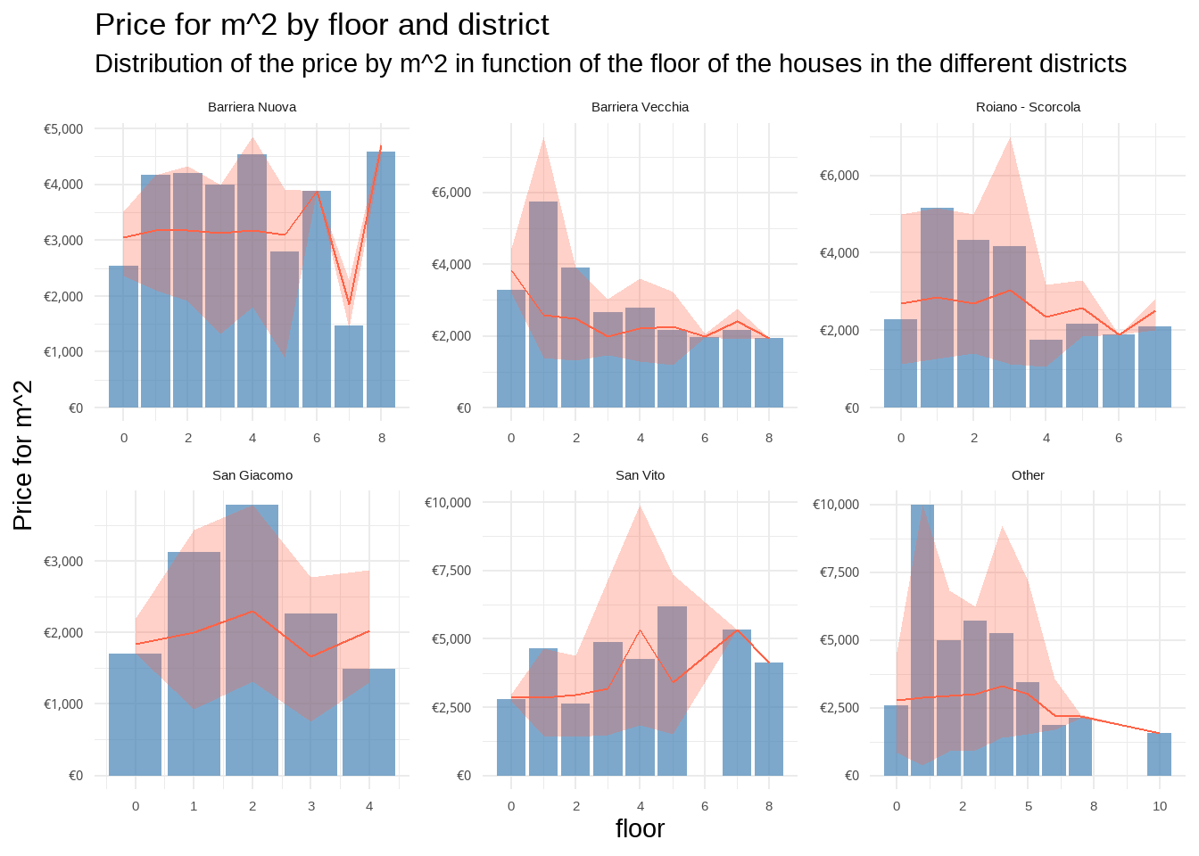
In this section, some plots are shown to give an idea of the data.
Plots
Code
data |>filter(!is.na(floor)) |>mutate(across(city_area, \(x) fct_na_value_to_level(x, "NA") |>fct_lump_n(5)) ) |>summarise(n =n(),across( priceByArea,list(max = max, min = min, mean = mean),.names ="{.col}_{.fn}" ),.by =c(floor, city_area) ) |># transform n to a range between min and max of priceByAreamutate(across( n, \(x) qunif( (x -min(x))/(max(x) -min(x)), priceByArea_min, priceByArea_max ) ),.by = city_area ) |>ggplot(aes(x = floor)) +# just to have pricebyarea in the y axisgeom_line(aes(y = priceByArea_mean),alpha =0, ) +# geom_ribbon(# aes(ymin = priceByArea_min, ymax = priceByArea_max),# fill = "tomato",# alpha = .3# ) +geom_col(aes(y = n),alpha = .7,fill ="steelblue", ) +geom_line(aes(y = priceByArea_mean),color ="tomato", ) +geom_ribbon(aes(ymin = priceByArea_min, ymax = priceByArea_max),fill ="tomato",alpha = .3 ) +facet_wrap(~city_area,ncol =3,scales ="free",labeller =label_wrap_gen() ) +scale_y_continuous(name ="Price for m^2",labels =~dollar(.x, prefix ="€"),# limits = ~ list(0, max(.) * 1.1),# sec.axis = sec_axis(trans = ~ . / max(.y), name = "Price") ) +scale_x_continuous(labels =~number(., accuracy =1) ) +labs(y ="",title ="Price for m^2 by floor and district",subtitle ="Distribution of the price by m^2 in function of the floor of the houses in the different districts", ) +theme_minimal()
Code
p = data |>filter(!is.na(floor), !is.na(size)) |>mutate(across(city_area, \(x) fct_na_value_to_level(x, "NA") |>fct_lump_n(8)) ) |>ggplot(aes(x = size, y = price, color = city_area,group = city_area, text = label)) +geom_point(alpha = .7,size =1, ) +geom_smooth(alpha = .9,se = F,linewidth = .5,linetype ="dashed", ) +scale_y_log10(labels = \(x) dollar(x, prefix ="€", suffix ="k",scale = .001, accuracy =1) ) +scale_x_continuous(limits =c(15,200), ) +# scale_x_log10() +theme(legend.position ="bottom",legend.title =element_blank(), ) +theme_minimal() +guides(color =guide_legend(nrow =2) ) +labs(x ="Size (m^2)",y ="Price",title ="Price of the houses in relation to the size",color ="District" )# interact the plotggplotly(p, tooltip ="text") |> plotly::layout(width =800, height =750, legend =list(orientation ="h", x =0.5, xanchor ="center", y =-0.2 ) )
Maps
Mappa del prezzo delle case nelle diverse zone della città. La mappa è interattiva, cliccando sui singoli pallini comparirà una box con ulteriori dati sulla casa.
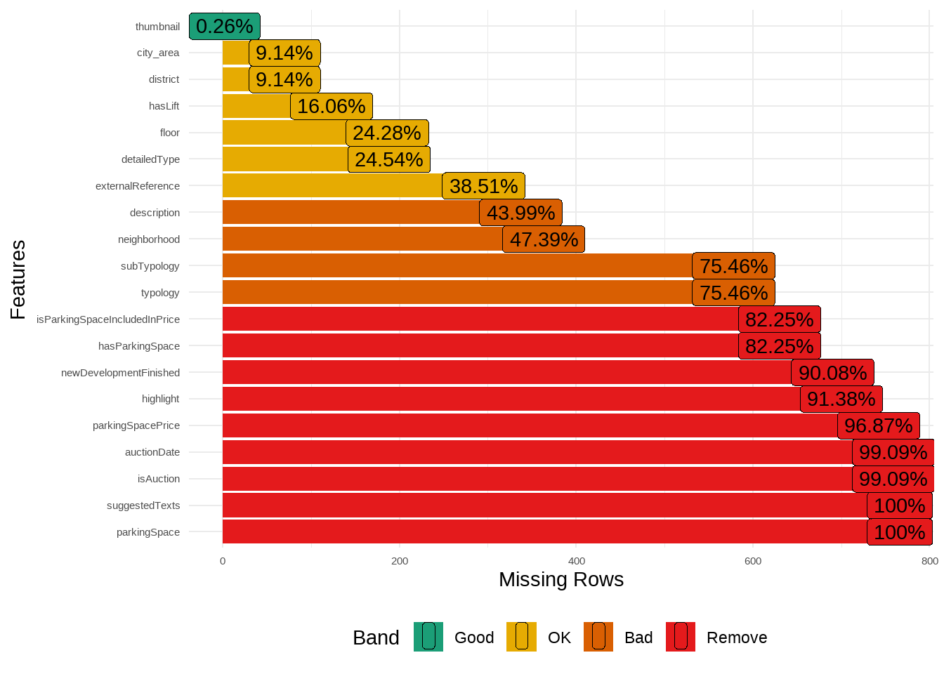
data |>select(# select only columns with less than 80% of NAs data |>summarise(across(everything(), \(x) sum(is.na(x)) /nrow(data)) ) |>pivot_longer(everything()) |>filter(value < .8) |>pull(name) ) -> data
Model
Pre processing
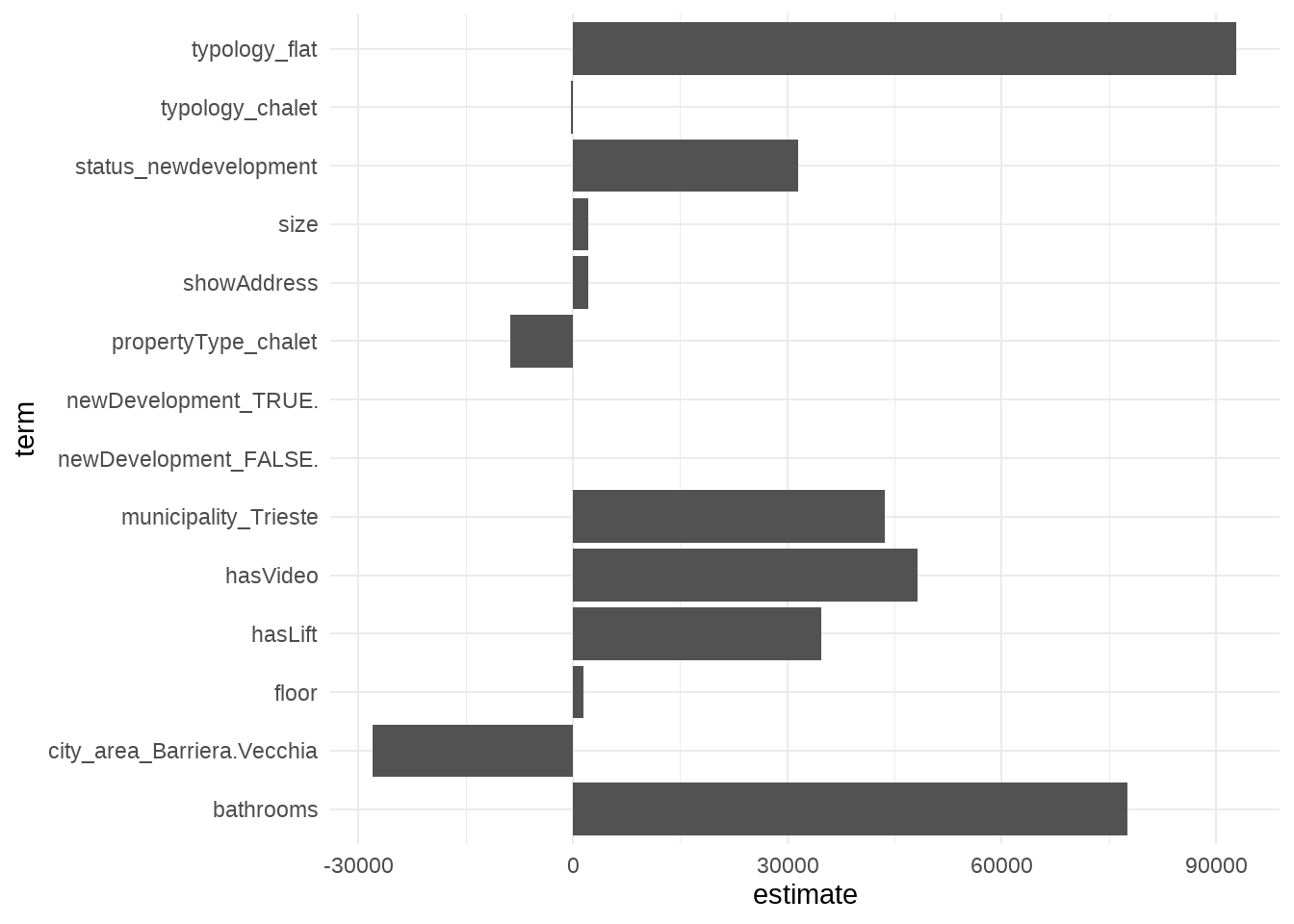
I develop an easy model to figure out how the variables for an ad influence the price posted on. I will use the {tidymodels} framework to deal it. The dataset will be splitted into 2 dataset, one for training and one for testing.
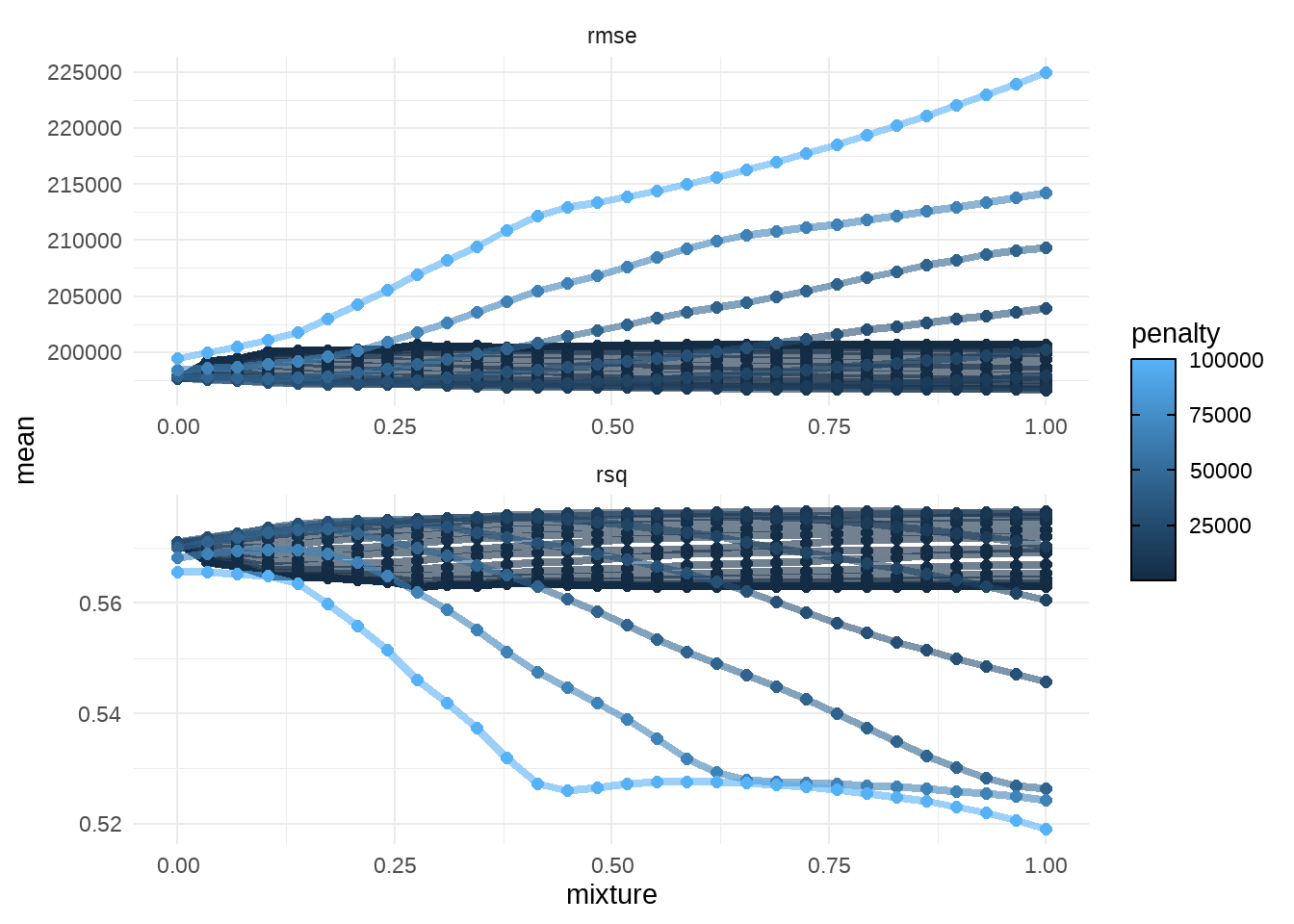
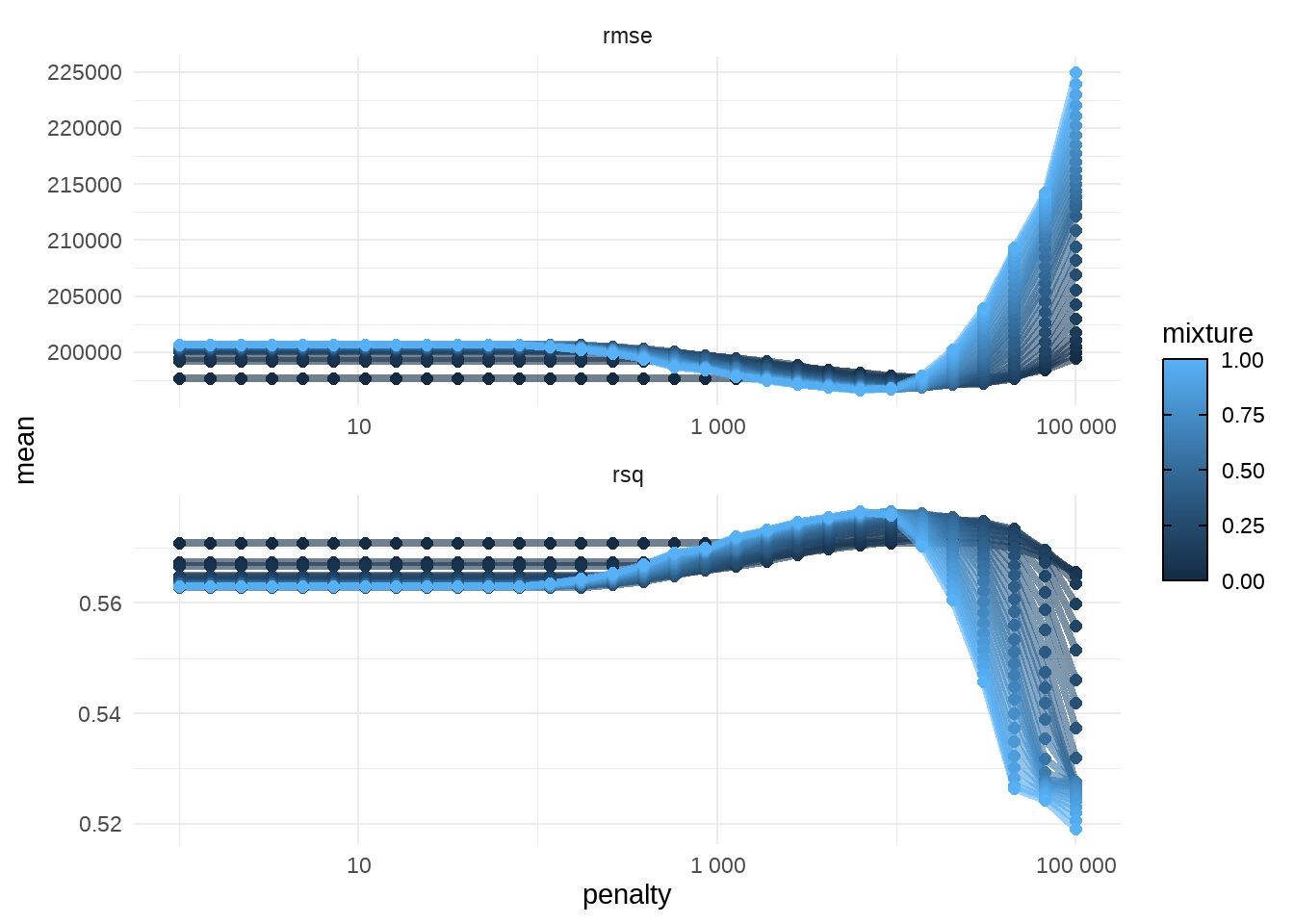
I use a penalized linear regression via {glmnet} package. I create a grid of parameters for penalty and mixture and I’ll train a model for each combination of parameters. After that I’ll estimate the metrics of the models and I’ll choice the best one based on RMSE (Root Mean Square Error).
Code
# set the modelmod <-linear_reg(penalty =tune(),mixture =tune() ) |>set_engine("glmnet")data_grid <-grid_regular(penalty(c(5, 0)),mixture(c(0, 1)),levels =30)# for the cross validationset.seed(1)data_folds <-vfold_cv(data_train, v =10)
In the recipe, there is the formula and the pre process rules. I remove all columns with low variance and group less common levels of the factor variables. For the nominal predictors who are NA I assign the unknown category while for numeric ones I impute the median of the category.
Code
# set the reciperec <-recipe(price ~ ., data = data) |># these items won't be bake. They could be useful for the future analysisupdate_role(propertyCode, latitude, longitude, url, description, priceByArea, title, label, new_role ="ID") |># remove unuseful featuresstep_rm(thumbnail, priceInfo, distance, externalReference, subtitle, neighborhood, district) |># logical to factorstep_mutate_at(all_logical_predictors(), fn =~as.numeric(.)) |># remove zero variance predictorsstep_zv(all_predictors()) |># remove features almost equalsstep_nzv(all_predictors(), freq_cut =95/5) |># for some levels who aren't present in training set but in testing setstep_novel(all_nominal_predictors()) |># add unknown to missing valuesstep_unknown(all_nominal_predictors()) |># group unfrequent classes to "other"step_other(all_factor_predictors(), threshold = .1) |># fill NAs who didn't manage them beforestep_impute_median(all_numeric_predictors()) |># NA omit# step_naomit(all_predictors()) |># step_dummy(all_logical_predictors(), one_hot = T) |> step_dummy(all_nominal_predictors(), one_hot = T) # reduce multicollinearity# step_corr(all_predictors(), threshold = .9, )workflow() |>add_model(mod) |>add_recipe(rec) -> wkflw# prep(rec, training = data_train) |> # bake(new_data = NULL)prep(rec, log_changes = T)
step_rm (rm_Hc7ab):
 removed (7): thumbnail, priceInfo, district, neighborhood, distance, ...

step_mutate_at (mutate_at_PL71w): same number of columns

step_zv (zv_OQv4A):
 removed (5): operation, province, country, topNewDevelopment, topPlus

step_nzv (nzv_ibiO2):
 removed (4): detailedType, has3DTour, has360, hasStaging

step_novel (novel_1EelD): same number of columns

step_unknown (unknown_lyXyh): same number of columns

step_other (other_V6alB): same number of columns

step_impute_median (impute_median_RlDvT): same number of columns

step_dummy (dummy_ZE3pu):
 new (24): propertyType_chalet, propertyType_flat, propertyType_other, ...
 removed (8): propertyType, address, municipality, status, ...
I assume that the model could estimate the real price, so in the table below are shown the price published with the delta from the price predicted. This is useful to check when an house is over or under estimated. The model doesn’t take in account the whole parameters which an house agency should take, so that this model is just to give a first prediction of the house price.